Sponsor

Senin, 11 Desember 2023

Utilizing VLOOKUP Across Different Sheets in Excel (Two Scenarios)

When grappling with extensive data scattered across various worksheets within your Excel workbook, the VLOOKUP function emerges as a valuable ally. Not only is VLOOKUP among the most useful functions in Excel, but it also stands out as one of the more intricate ones. This function proves instrumental in consolidating data from multiple sheets in a coherent manner. This article delves into the nuances of employing the VLOOKUP function from another sheet in Excel, covering two distinct cases.

Introduction to the VLOOKUP Function in Excel

In straightforward terms, the VLOOKUP function takes user-input, searches for it within the Excel worksheet, and retrieves a corresponding value associated with the given input. This functionality spans across all versions of Excel, starting from Excel 2007.

Key Points


The VLOOKUP function processes the input value, scans the worksheets for a match, and furnishes the corresponding value.

Syntax

=VLOOKUP(lookup_value, table_array, col_index_num, [range_lookup])

Argument


Result

Yields an exact or approximate value corresponding to the user's provided input.

Utilizing VLOOKUP Across Different Sheets: Two Scenarios


Applying the VLOOKUP function to retrieve values can involve two distinct scenarios—either from a single alternative worksheet or multiple worksheets. Below, we'll illustrate these two cases.

Case 1: VLOOKUP from Another Single Sheet


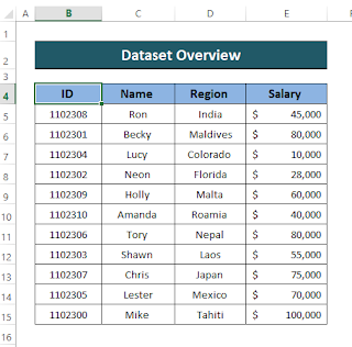
Here, we'll explore how to employ the VLOOKUP function when extracting data from a separate sheet within the same workbook. Consider a dataset featuring "ID" numbers, Sales Reps' "Names," "Regions," and "Salaries," as shown in the provided image. In this dataset, the ID numbers are assigned arbitrarily, and our objective is to place the ID number in a different worksheet and extract the associated information.

🔗 Steps:

1. Begin by creating a new worksheet where you intend to retrieve information matching the ID number using the VLOOKUP function.

2. Apply the VLOOKUP function in the Name Column:

   =VLOOKUP(B5, 'Employee Data'!B$5:E$15, 2, FALSE)

   - Lookup_value is B$5
   - table_array is 'Employee Data'!B$5:E$15 (Select the array from the employee data worksheet)
   - Col_index_num is 2
   - [range_lookup] is set to FALSE for an exact match.

3. Press "ENTER" to obtain the value from another worksheet.

4. Select the cell containing the function, and using the Fill Handle, drag downward to Autofill the formula into the subsequent cells.

5. As a result, you will get the same result for the rest of the ID numbers.

   *Note: The lookup range, 'B$4:E$14,' indicates a locked column, ensuring that cell references won't change when copying or dragging the formula. Using absolute cell reference ($B$4:$E$14) would freeze both the row and column.*

6. Hold the Fill Handle, select the column Name, and drag the mouse to the right-end corner to populate the remaining results.

By following these steps, all subsequent cells will auto-fill with the VLOOKUP function, providing the desired results for the remaining ID numbers.

2. VLOOKUP Across Multiple Sheets


When the need arises to search for values across two or more sheets, the earlier method may not be the most convenient. The optimal solution involves employing the VLOOKUP function with nested IFERROR or Nested INDIRECT functions to systematically search between worksheets. Let's delve into this technique.

2.1. Utilizing the IFERROR Function


Consider a scenario where we have three worksheets containing employee data from the "India," "Nepal," and "Japan" regions. 


Our goal is to locate their salary in a new worksheet using their ID number as input, employing VLOOKUP nested within the IFERROR function. The formula format is as follows:

=IFERROR(VLOOKUP(…), IFERROR(VLOOKUP(…), …, "Not found"))

If no value is found, the formula gracefully returns "NOT FOUND".

🔗 Steps:

1. Begin by creating a new worksheet featuring the ID number and Salary column. Input the desired ID number in the ID column.


2. Apply the following formula containing VLOOKUP with the IFERROR function:

   =IFERROR(VLOOKUP(B5, India!$B$5:$E$10, 4, FALSE), IFERROR(VLOOKUP(B5, Nepal!$B$5:$E$10, 4, FALSE), IFERROR(VLOOKUP(B5, Japan!$B$5:$E$10, 4, FALSE), "NOT FOUND")))

   - Lookup_Value is B5
   - Sheet_range includes India!$B$5:$E$10, Nepal!$B$5:$E$10, Japan!$B$5:$E$10
   - Col_index_num is 4
   - Range_lookup is set to False for an Exact Match


3. Press ENTER to retrieve the value.


4. Copy the formula for the remaining cells.


Upon inspection, in the case of ID number "1102316," the value is "NOT FOUND" since this ID number does not exist in the specified worksheets. Thus, the VLOOKUP from another sheet in Excel is successfully executed using this approach.


2.2. Utilizing the INDIRECT Function


An alternative method for VLOOKUP across multiple sheets in Excel involves a combination of the "VLOOKUP" and "INDIRECT" functions, alongside INDEX, MATCH, and COUNTIF functions. Introducing an additional worksheet named "Africa" alongside the three lookup sheets mentioned in Method 2.1, let's explore this approach.


Now, let's consider four distinct worksheets containing employee information and apply the following formula on a new compilation worksheet:

=VLOOKUP(lookup_value, INDIRECT("'" & INDEX(Lookup_sheets, MATCH(1, --(COUNTIF(INDIRECT("'" & Lookup_sheets & "'!lookup_range"), lookup_value)>0), 0)) & "'!table_array"), col_index_num, FALSE)

🔗 Steps:

1. Name the worksheets as "India," "Nepal," "Japan," and "Africa." Write down all the lookup sheet names in any cell of your workbook and name that range.


2. Apply the following formula:

   =VLOOKUP($B5, INDIRECT("'" & INDEX(Lookup_Sheets, MATCH(1, --(COUNTIF(INDIRECT("'" & Lookup_Sheets & "'!$B$5:$B$10"), $B5) > 0), 0)) & "'!$B$5:$E$10"), 4, FALSE)

   - Lookup_value is $B5.
   - Lookup_sheets is the named range containing the names of the sheets.
   - Lookup_range is the column range to look up for ($B$5:$B$10).
   - Table_array is the data range ($B$5:$E$10).
   - Col_index_num is 4.
   - "FALSE" is for the exact match.


3. This is an array formula, so press SHIFT+CTRL+ENTER simultaneously to apply.

💡 Formula Explanation:

The segment `INDIRECT("'" & INDEX(Lookup_Sheets, MATCH(1, --(COUNTIF(INDIRECT("'" & Lookup_Sheets & "'!$B$5:$B$10"), $B5) > 0), 0)) & "'!$B$5:$E$10")` serves as the lookup array for the VLOOKUP function. Let's break it down.

- `Lookup_sheets` is a named range with values: India, Nepal, Japan, Africa.

- `INDIRECT("'" & Lookup_Sheets & "'!$B$5:$B$10")` returns an array: {1102304; 1102310; 1102314; 1102320}.
- `COUNTIF(INDIRECT("'" & Lookup_Sheets & "'!$B$5:$B$10"), $B5)` results in an array: {1; 0; 0; 0}.

- `MATCH(1, --(COUNTIF(INDIRECT("'" & Lookup_Sheets & "'!$B$5:$B$10"), $B5) > 0), 0)` equals 1.
- `INDEX(Lookup_Sheets, MATCH(1, --(COUNTIF(INDIRECT("'" & Lookup_Sheets & "'!$B$5:$B$10"), $B5) > 0), 0))` returns "India."

Now, the formula becomes `VLOOKUP($B5, INDIRECT("'" & "India" & "'!$B$5:$E$10"), 4, FALSE)`. 

`INDIRECT("'" & "India" & "'!$B$5:$E$10")` fetches the array $B$5:$E$10 from the India sheet, resulting in: {1102304,"Ronand","India",44000; 1102302,"Duke","India",56000; ...}.

The final output is $12000, corresponding to the given ID number. Repeat this formula for the remaining IDs. Non-existing IDs will yield "#N/A."

💡 Things to Remember:

- The VLOOKUP function searches for lookup values from the leftmost top column to the right.
- A column index number less than 1 will result in an error.
- Use absolute cell references ($) for the "Table_Array".
- Press SHIFT+CTRL+ENTER for array formulas.

Download the Practice Workbook


Feel free to download the accompanying practice sheet to reinforce your understanding as you go through this article.


Conclusion


This article has covered the process of searching for data in one or multiple worksheets and organizing them systematically using the VLOOKUP function from another sheet. While this function may pose a challenge for new users, we've aimed to simplify the explanation as much as possible. We hope this article proves useful for you. If you encounter any confusion, please share your thoughts, and we'll be happy to assist.

Automating Formula AutoFill in Excel with VBA: A Comprehensive Guide (5 Practical Examples)

If you've been navigating Microsoft Excel for some time, you're likely familiar with the indispensable function of AutoFill. While manually using the mouse to copy a formula across rows or columns is feasible for smaller datasets, the process becomes cumbersome with larger sets of data. Enter Visual Basic for Applications (VBA) – a powerful tool that allows you to seamlessly AutoFill a formula to the last row or column with precision and efficiency.

In this tutorial, we will delve into the world of VBA codes, providing you with clear examples and illustrations on how to automate the AutoFill process in Excel. Let's explore the power of VBA to enhance your workflow.

Before we dive into the VBA magic, let's briefly revisit what AutoFill is in Excel. AutoFill is an in-built feature in Microsoft Excel designed to automatically populate the remaining rows or columns with values, formats, or formulas. You can easily spot it by moving your cursor to the lower-right corner of any cell – this nifty feature is known as the AutoFill handler.

Now, let's proceed with the VBA journey to effortlessly AutoFill formulas to the last row in Excel. Stay tuned for insightful examples and step-by-step guidance.

Understanding AutoFill in Excel:


AutoFill is an inherent capability within Microsoft Excel, empowering users to effortlessly populate the remaining rows or columns with values, formats, or formulas. Recognition of this feature is simple – just position your cursor in the lower-right corner of any cell, commonly referred to as the AutoFill handler.

Refer to the accompanying screenshot:
Basic autofill

In the provided example, observe two numbers in cells B5 and B6. Our goal is to extend this sequence to fill the subsequent rows using the AutoFill feature in Excel.

Commence by selecting the range of cells from B5 to B6. Subsequently, locate the AutoFill handle positioned in the lower-right corner.

Upon identifying the AutoFill handle, drag it downward.

Witness Excel's automatic population of the remaining cells in the column. This exemplifies the fundamental application of the AutoFill feature in Excel.

Utilizing AutoFill with Excel VBA:


When dealing with an extensive number of rows or columns within a specific range, manually dragging down the AutoFill handle to reach the last row or column can be a cumbersome task. Fortunately, this can be streamlined using VBA codes in Excel. VBA allows you to efficiently AutoFill cells with values, formulas, or formats, simplifying the process.

The Generalized Syntax:

Range.AutoFill Destination, Type

Here's the breakdown:

- Range(“B5”): Refers to the cell containing the primary pattern to be extended throughout the series.

- Destination: Denotes the range of cells where the pattern series is to be filled.

- Type as xlAutoFillType: Specifies the type of series fill. Various AutoFill types are available for selection, providing flexibility in the AutoFill process.


Exploring 4 AutoFill Types in Excel VBA:


In this segment, we will delve into various types of AutoFill in Excel VBA. As mentioned earlier, the xlAutoFillType parameter allows us to select different AutoFill types. Let's explore some examples:

1. xlFillDefault:

In our previous example, we encountered this AutoFill type.

Observe the provided screenshot:

Utilize the following VBA code to AutoFill the remaining cells:

Sub xlDefault_type()

Range("B5:B6").AutoFill Destination:=Range("B5:B11"), Type:=xlFillDefault

End Sub

Execute the VBA macro, and the outcome will be as follows:

Witness the automatic population of the remaining cells facilitated by the VBA macro.

2. xlFillCopy:

For duplicating identical values, the xlFillCopy type in the AutoFill category can be employed.

Refer to the provided screenshot:

Insert the following VBA code to automatically fill the remaining cells:

Sub xlFillCopy_type()
    Range("B5:B6").AutoFill Destination:=Range("B5:B11"), Type:=xlFillCopy
End Sub

Execute the VBA macro, and the result will be as follows:
Excel seamlessly populates the remaining cells with the identical pattern of values.

3. xlFillMonths:

To populate cells with months, leverage the xlFillMonths AutoFill type.

Refer to the accompanying screenshot:
In this example, we've inputted two months, January and February.

Insert the following VBA code to AutoFill the remaining cells:

Sub xlFillMonths_type()
    Range("B5:B6").AutoFill Destination:=Range("B5:B11"), Type:=xlFillMonths
End Sub

Execute the VBA macro, and the outcome will be as follows:
Excel intelligently discerns the month patterns and seamlessly fills the cells accordingly.

4. xlFillFormats:


To replicate formats across cells using VBA AutoFill, employ the xlFillFormats AutoFill type.

Examine the provided screenshot:
In this instance, two cells have been adorned with distinct colors.

Now, input the following VBA code to AutoFill the remaining cells:

Sub xlFillFormats_type()
    Range("B5:B6").AutoFill Destination:=Range("B5:B11"), Type:=xlFillFormats
End Sub

Execute the VBA macro, and the result will be as follows:
As evident, our VBA macro adeptly utilizes AutoFill to efficiently propagate the formatting across the rows of column B.

Automating Formula AutoFill in Excel with VBA: A Comprehensive Guide (5 Practical Examples)


1. VBA for AutoFilling a Formula to the Last Used Row:


Similarly, leveraging VBA enables you to effortlessly AutoFill a formula, building upon the concepts discussed in preceding sections. The challenge arises when you need to extend the formula to the last used row. This necessitates identifying the last used row before implementing the VBA code to execute the AutoFill.

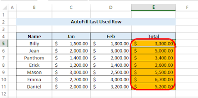
Consider the provided dataset:

In this scenario, we have a sales dataset featuring salespersons. The objective is to sum the sales of January and February, adding the results to the Total column. Subsequently, we will utilize the VBA AutoFill method to propagate this formula to the last used row in Excel.

To achieve this, input the following code:

Sub last_used_row()

Dim last_row As Long

last_row = Cells(Rows.Count, 2).End(xlUp).Row

Range("E5").Formula = "=SUM(C5:D5)"

Range("E5").AutoFill Destination:=Range("E5:E" & last_row)

End Sub

Explanation of key components:

- last_row = Cells(Rows.Count, 2).End(xlUp).Row: Determines the last used row in column B. You can adapt this to any column in your dataset.

- Range("E5").Formula = "=SUM(C5:D5)": Adds the sales of cells C5 and D5.

- Range("E5").AutoFill Destination:=Range("E5:E" & last_row): After obtaining the result, the AutoFill function starts from cell E5 and extends to the last used row obtained earlier.

Execute the VBA macro, and observe the resulting output:

As evident, our VBA code effectively sums the initial result and AutoFills the formula to the last row in Excel.

2. VBA AutoFill from ActiveCell to Last Row:


If you prefer not to specify a particular range in the AutoFill method and instead utilize the values, formulas, or formats of the active cell, this approach allows for seamless automation. This is particularly handy when you want to AutoFill the rest of the rows with the active cell's formula by simply clicking on a cell.

It is similar to the previous example. We are using the previous dataset:


Let's illustrate this with an example of adding the sales of January and February, AutoFilling the formula to the last row using Excel VBA. Execute the following code:

Sub autofill_active_cell()

Dim last_row As Long

last_row = Cells(Rows.Count, 2).End(xlUp).Row

ActiveCell.Formula = "=SUM(C5:D5)"

ActiveCell.AutoFill Destination:=Range(ActiveCell.Address & ":E" & last_row)

End Sub

Explanation of key components:

- last_row = Cells(Rows.Count, 2).End(xlUp).Row: Determines the last used row in column B. You can adapt this to any column in your dataset.

- ActiveCell.Formula = "=SUM(C5:D5)": Adds the sales of cells C5 and D5 to the selected cell.

- ActiveCell.AutoFill Destination:=Range(ActiveCell.Address & ":E" & last_row): After obtaining the result, the AutoFill function starts from the active cell and extends to the last used row obtained earlier.

Here's a simple step-by-step guide:

1. Select Cell E5.

2. Run the VBA macro to add the formula and AutoFill it to the last row.

As illustrated, the VBA macro has successfully AutoFilled the formula to the last row, utilizing the active cell as the starting point.

3. Dynamic Range AutoFill to Last Row with Excel VBA:


In our previous discussions, we shared VBA macros for AutoFilling to the last row in Excel. However, in those examples, we exclusively employed dynamic ranges.

Let's examine a scenario involving static ranges for a better understanding:

Sub last_used_row()

Range("E5").Formula = "=SUM(C5:D5)"

Range("E5").AutoFill Destination:=Range("E5:E11")

End Sub

In this instance, we instructed Excel to input a formula in Cell E5 and AutoFill it from Cell E5 to Cell E11. Here, the range was explicitly specified. The drawback arises when additional rows are added; the VBA won't AutoFill those extra rows since we predefined a specific range.

To overcome this limitation, we've devised a solution that accommodates dynamic ranges:

Sub last_used_row()

Dim last_row As Long

last_row = Cells(Rows.Count, 2).End(xlUp).Row

Range("E5").Formula = "=SUM(C5:D5)"

Range("E5").AutoFill Destination:=Range("E5:E" & last_row)

End Sub

As illustrated, we first determine the last row using this line of code:

last_row = Cells(Rows.Count, 2).End(xlUp).Row

Subsequently, we AutoFill to the last row using the dynamic range:

Range("E5").AutoFill Destination:=Range("E5:E" & last_row)

This VBA code adeptly identifies the number of rows in your dataset, ensuring successful AutoFill with the formula, regardless of how many rows you add.

In essence, a dynamic range eliminates the need to manually input the range, allowing Excel to automatically update it as needed.


4. AutoFill to Last Column in Excel Using VBA:


If you've followed the earlier sections on AutoFilling to the last row, extending the functionality to the last column using Excel VBA is a straightforward process. By identifying the last column number, you can effortlessly AutoFill the formula.

Consider the provided dataset:

In this dataset, we're representing a 3-month budget. Our objective is to sum the expenses for all months and AutoFill the formula to the last column using Excel VBA.

Execute the following code:

Sub last_used_column()

Dim last_column As Long

last_column = Cells(6, Columns.Count).End(xlToLeft).Column

Range("D9").Formula = "=SUM(D6:D8)"

Range("D9").AutoFill Destination:=Range("D9", Cells(9, last_column))

End Sub

Explanation of key components:

- last_column = Cells(6, Columns.Count).End(xlToLeft).Column: Determines the last used column from row 6. You can customize the starting row based on your dataset.

- Range("D9").Formula = "=SUM(D6:D8)": Adds the expenses of three months (Jan, Feb, Mar).

- Range("D9").AutoFill Destination:=Range("D9", Cells(9, last_column)): After obtaining the result, the AutoFill function starts from column D and extends to the last used column identified by `last_column`. The main row is Row 9, containing all our data.

Upon running the macro, observe the resulting output:

The VBA has effectively AutoFilled the formula to the last column in Excel, demonstrating the seamless extension of functionality from rows to columns.

5.  AutoFill Sequential Numbers to Last Row in Excel with VBA:


You can effortlessly AutoFill sequential numbers in Excel using VBA, specifically by employing `xlFillSeries` as the AutoFill type. Excel intelligently recognizes the pattern and seamlessly populates the cells accordingly.

Consider the dataset presented in the following screenshot:

In this example, we have a list of names, and the goal is to assign sequential IDs to them using VBA AutoFill.

AutoFill Sequential Numbers with a Static Range:

Sub sequential_number_2()

Range("C5").AutoFill Destination:=Range("C5:C11"), Type:=xlFillSeries

End Sub

After executing the code, observe the output:

If you prefer a dynamic range, utilize the following code:

Sub sequential_number_1()

Dim last_row As Long

last_row = Cells(Rows.Count, 2).End(xlUp).Row

Range("C5").AutoFill Destination:=Range("C5:C" & last_row), Type:=xlFillSeries

End Sub

Here, 

last_row = Cells(Rows.Count, 2).End(xlUp).Row: determines the last used row in column B.

Range("C5").AutoFill Destination:=Range("C5:C" & last_row), Type:=xlFillSeries: takes the ID from Cell C5 and AutoFills it to the last used row in Column C using `xlFillSeries`.

In both cases, the outcome remains consistent:

As demonstrated, the VBA code effectively AutoFills sequential numbers in Excel.

Download Practice Workbook

Conclusion:


In conclusion, this tutorial aims to equip you with valuable knowledge on AutoFilling formulas to the last row using VBA codes. We encourage you to practice these instructions on your dataset by downloading the provided workbook. Feel free to experiment and provide feedback in the comments. Your input motivates us to create more tutorials.

Embrace continuous learning and growth!